1.KAGGLE의 IMDB 영화평 지도 학습 기반
=> url - https://www.kaggle.com/c/word2vec-nlp-tutorial/data
Bag of Words Meets Bags of Popcorn | Kaggle
www.kaggle.com
=>데이터 구조:id (유저의 아이디), sentiment(감성으로 긍정이 1 , 부정이 0), review(리뷰)
이 경우는 레이블이 있는 데이터를 가지고 범주를 예측하는 것과 동일
자연어는 피처가 문장으로 주어지기 떄문에 문장을 피처 벡터화 작업을 해주는 것이 다릅니다.
이 때 모든 단어를 각각의 피처로 만들고 각 문장은 피처의 존재 여부를 데이터로 소유합니다.
자연어 처리에서 feature 를 만드는 방법이 다른데 , 영어는 word_tokenize 하고 불용어를 제거하면 되지만, 한국어는 형태소분석 후 word_tokenize 하고 불용어를 제거합니다. 근데 성능은 형태소 분석을 하고 나서 성능이 더 좋게 발휘됩니다.
=>데이터 전처리
- <br />를 제거:replace
- 영문만 남겨두기:정규식 모듈의 sub 메서드를 활용
#데이터 전처리
#<br /> 제거
review_df['review'] = review_df['review'].str.replace("<br />"," ")

#영문자가 아닌 단어들 모두 제거
#a-zA-Z 가 아닌 글자를 공백으로 치환
#한글을 제외한 글자 제거 :[^가-힣]
import re
review_df['review'] = review_df['review'].apply(lambda x : re.sub("[^a-zA-Z]"," ",x))

print(review_df['review'].head())

아래와 같이 영문자가 아닌 단어들을 모두 제거
=>지도 학습 기반의 분류이므로 훈련 데이터를 이용해서 훈련을 하고 테스트 데이터로 확인하는 것을 권장하기 때문에 데이터를 분리
#훈련 데아터와 검증 데이터 분리

from sklearn.model_selection import train_test_split

class_df = review_df['sentiment']
feature_df = review_df.drop(['id','sentiment'],axis=1,inplace =False)

X_train, X_test, y_train, y_test = train_test_split(feature_df,class_df ,test_size=0.3,random_state=42)
print(X_train.shape)
print(X_test.shape)
=>CountVectorizer 로 피처 벡터화를 수행한 후 분류 모델을 훈련
#CountVectorizer를 이용한 피처 벡터화 후 분류 모델 훈련

pipeline = Pipeline([
    ('cnt_vect',CountVectorizer(stop_words='english',ngram_range=(1,2))),
    ('lr_clf',LogisticRegression(C=10))
])

pipeline.fit(X_train['review'],y_train)
pred = pipeline.predict(X_test['review'])


pred_probs = pipeline.predict_proba(X_test['review'])
acc=accuracy_score(y_test,pred)#정확도는 pred
roc = roc_auc_score(y_test,pred_probs)# roc_auc 줄때는 확률을 줘야함
print("정확도:",acc)
print("roc-auc:",roc)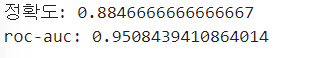
ngram 은 기본적으로 하나의 단어를 하나로 인식하지만, ngram을 설정해주면 몇 개의 단어까지 하나의 단어로 인지할 수 있는지를 설정. 영문에서는 2나 3을 설정합니다. 2는 사람이름의 영어권은 2나 3 정도 되기 때문이기도 하고, 사람 이름이 많이 등장하는 경우는 직급도 포함하는경우가 많기 때문입니다.
ngram을 설정해야 더 좋은 예측하게 됩니다.
=>TdidfVectorizer로 피처 벡터화를 수행한 후 분류 모델을 훈련 =>이게 보편적으로 더 좋음
#TfidfVectorizer를 이용한 피처 벡터화 후 분류 모델 훈련

pipeline = Pipeline([
    ('cnt_vect',TfidfVectorizer(stop_words='english',ngram_range=(1,2))),
    ('lr_clf',LogisticRegression(C=10))
])

pipeline.fit(X_train['review'],y_train)
pred = pipeline.predict(X_test['review'])


pred_probs = pipeline.predict_proba(X_test['review'])[:,1]
acc=accuracy_score(y_test,pred)#정확도는 pred
roc = roc_auc_score(y_test,pred_probs)# roc_auc 줄때는 확률을 줘야함
print("정확도:",acc)
print("roc-auc:",roc)
2.비지도 학습 기반 감성 분석
=>레이블이 없는 경우 사용
=>Lexicon이라는 감성 분석에 관련된 어휘집을 이용하는 방식
=>한글 버전의 Lexicon이 현재는 제공되지 않음
네이버의 식당 리뷰 감성 분석:이진 분류는 LogisticRegression이면 충분
=>데이터는 크롤링한 데이터: review_data.txt 파일
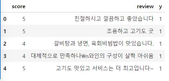
=>내용은 score 와 review 와 y로 구성
score 은 별점이고 y 가 감성인데 score 가 4이상이면 1 그렇지 않으면 0으로 라벨링
=>데이터 읽어오기
df = pd.read_csv('./review_data.csv')
df.info()
df.head()
숫자랑 \n같은 기호를 없애야함
=>데이터 전처리
-한글 추출: 이전에는 한글 글자만 추출(가-힣을 많이 했는데 최근에는 모음 과 자음만으로 구성된 텍스트(ㄱ-ㅣ 가-힣)도 추출
이런건 함수로 만들어놓고 쓰는게 좋음
#한글을 제외한 글자를 전부 제거하기

def text_cleaning(text):
    hangul = re.compile('[^ㄱ-ㅑ 가-힣]')
    result = hangul.sub('',text)
    return result

df['ko_text'] = df['review'].apply(lambda x:text_cleaning(x))
del df['review']
df.head()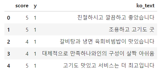
del은 메모리까지 정리해줘서 좋음.
-한글을 사용할 떄는 토큰나이저를 이용하지 않고 형태소 분석을 수행해서 사용합니다
#형태소 분석

from konlpy.tag import Okt

#문장을 받아서 형태소 분석을 수행해서 결과를 리턴해주는 함수
#단어와 품사를 이전처럼 / 로 구분해서 리턴
def get_pos(x):
    tagger= Okt()
    pos = tagger.pos(x)
    pos = ['{}/{}'.format(word,tag) for word, tag in pos]
    return pos
-feature 벡터화: 등장하는 모든 단어를 수치화시키는 작업
#등장 횟수만을 고려한 피처 벡터화를 위한 사전 생성
from sklearn.feature_extraction.text import CountVectorizer

index_vectorizer = CountVectorizer(tokenizer = lambda x: get_pos(x))
X=index_vectorizer.fit_transform(df['ko_text'].tolist())
X.shape
#3016이 단어의 개수
#545는 행의 개수
'친절하시고 깔끔하고 좋았습니다'를 각 단어의 등장횟수로 인덱스로 변환

# CountVectorizer 를 이용해서 만든 피처 벡터를 Tfidf 기반으로 변경
from sklearn.feature_extraction.text import TfidfTransformer

tfidf_vectorizer=TfidfTransformer()
X= tfidf_vectorizer.fit_transform(X)
print(X)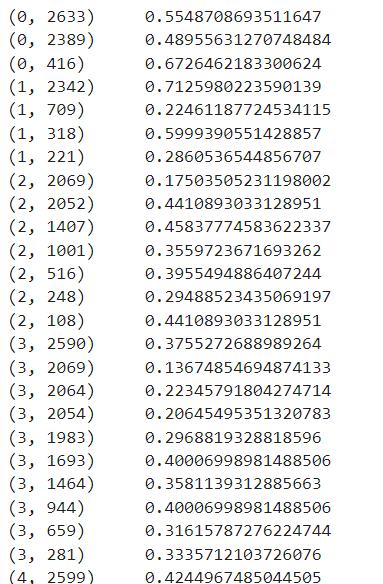
필요하다면 데이터를 제거하거나 추가를 해도 됩니다.
제거는 많이하고 추가는 예측할 데이터가 들어오면 그 데이터를 추가하는 형태로 작업
#훈련 데이터와 검증 데이터 생성

from sklearn.model_selection import train_test_split

y= df['y']
X_train, X_test, y_train, y_test = train_test_split(X,y,test_size=0.3,random_state=42)
print(X_train.shape)
print(X_test.shape)
#모델 생성및 훈련과 평가

from sklearn.linear_model import LogisticRegression
from sklearn.metrics import accuracy_score,recall_score,precision_score,f1_score

lr = LogisticRegression(random_state=42)
lr.fit(X_train, y_train)

y_pred = lr.predict(X_test)
y_pred_probability = lr.predict_proba(X_test)

print("정확도:",accuracy_score(y_test,y_pred))
print("precision:",precision_score(y_test,y_pred))
print("recall:",recall_score(y_test,y_pred))
print("f1:",f1_score(y_test,y_pred))
결과는 위와 같이 나오는데 , recall 값이 1이 나오는게 의심됨.이런 경우 confusion matrix로 확인한번 해보는게 좋음
#recall이 1인게 의심스러워서 confusion_matrix

from sklearn.metrics import confusion_matrix

print(confusion_matrix(y_test,y_pred))
모든 데이터를 다 긍정으로 예측함. 잘못된 모델이라고 볼 수 있음.데이터의 편차가 너무 심함을 알 수 있음. 아프리카에서 맑은 날씨라고 하면 당연히 맞출 확률이 높음.
-감성분석이나 신용 카드 부정 거래 탐지등을 수행할 때 주의할 점은 샘플의 비율이 비슷하지 않다는 것입니다.
일정한 비율을 가지고 샘플링 하는 것을 고려해야 합니다.
#타겟의 분포 확인

df['y'].value_counts()
1과 0의 비율이 10배 정도라 1을 언더 샘플링을 하던지, 0을 오버 샘플링 하는 것이 좋습니다.
#1의 개수를 줄여서 샘플링

positive_random_idx = df[df['y']==1].sample(50,random_state=42).index.tolist()
negative_random_idx = df[df['y']==0].sample(50,random_state=42).index.tolist()
print(positive_random_idx)

random_idx = positive_random_idx + negative_random_idx

#비율을 맞춘 데이터 생성
sample_X = X[random_idx,:]
y=df['y'][random_idx]
#모델 생성및 훈련과 평가
from sklearn.linear_model import LogisticRegression
from sklearn.metrics import accuracy_score,recall_score,precision_score,f1_score
lr = LogisticRegression(random_state=42)
lr.fit(X_train, y_train)
y_pred = lr.predict(X_test)
y_pred_probability = lr.predict_proba(X_test)
print("정확도:",accuracy_score(y_test,y_pred))
print("precision:",precision_score(y_test,y_pred))
print("recall:",recall_score(y_test,y_pred))
print("f1:",f1_score(y_test,y_pred))
recall값이 엄청 떨어진 것을 볼 수 있음
=>feature 별 중요도 확인
#feature 의 중요도 확인
#트리 계열 모델들은 feature_importances_라는 속성에 각 피처의 중요도를 가지고 있으
#트리 계열이 아닌 모델들은 회귀 계수를 가지고 판단
#모델의 회귀 계수는 coef_ 라는 속성에 저장됩니다
#각 피처에 대한 회귀 계수 - 단어
print(lr.coef_[0])

#회귀 계수 내림차순 정렬
coef_pos_index = sorted (((value,index) for index,value in enumerate(lr.coef_[0])),
                        reverse=True)

print(coef_pos_index)
'Study > Machine learning,NLP' 카테고리의 다른 글
| NLP(3)-문서 군집화,연관분석,추천시스템 (0) | 2024.03.14 |
|---|---|
| NLP(1)- 자연어 처리 (0) | 2024.03.13 |
| 머신러닝(10)-군집 (0) | 2024.03.11 |
| 머신 러닝(9)-차원 축소 (0) | 2024.03.07 |
| 머신러닝(8)-실습(2) (0) | 2024.03.07 |


